How to Read an Air Quality Assessment Report

Emissions, meteorology, dispersion modelling and Alberta regulatory requirements explained: An air quality assessment report connects what a facility emits to what people and the environment may experience at ground level and demonstrates whether those predicted concentrations meet applicable regulatory requirements.

It presents calculations of hourly and short-term emissions, predicts resulting air concentrations, and compares them against regulatory limits such as Alberta Ambient Air Quality Objectives (AAAQOs) and Guidelines (AAAQGs).

I also indicate how these things are handled in neighbouring provinces for comparison.

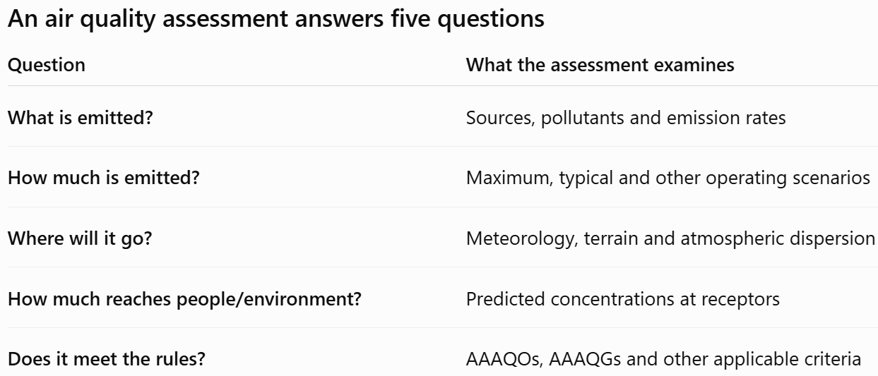
Why Read an Air Quality Assessment Report?

Industrial emissions and the environment

An air quality assessment report shows how industrial emissions affect air quality, public health, and regulatory compliance.

Using hourly weather data and dispersion models such as AERMOD, the report predicts where pollutants will travel, how concentrated they will become, and whether they meet air quality standards. It evaluates both typical and maximum operating conditions because facilities must remain compliant during normal operations, even when short-term emission spikes occur.

The report also explains:

• How pollutants disperse through the atmosphere
• How emissions affect nearby communities and the environment
• How sulphur compounds and odours are managed, including Total Reduced Sulphur (TRS)
• How short-term emission spikes are assessed against air quality limits
• How industrial growth, emissions, and environmental policy interact
• How operators maintain compliance with air quality regulations

At its core, an Air Quality Assessment connects industrial emissions to real-world environmental impacts and demonstrates how facilities manage air quality risks responsibly.

Alberta Air Quality Modelling: Emission Scenarios, Odour, and Compliance

An air quality assessment is more than running a dispersion model. The real challenge is selecting realistic emission scenarios, choosing appropriate assumptions, and demonstrating regulatory compliance.

To support regulatory approval, air quality assessment reports typically include:

• Predicted concentration tables
• Concentration contour maps
• Model input and control files
• Assumptions, methods, and supporting calculations

See Appendices A and B of the Alberta dispersion modelling guideline for examples.  The objective is to provide enough detail for the regulator to understand, reproduce, and approve the assessment without delays.

Typical vs. Maximum Emissions: Alberta often requires modelling of both maximum and typical operating conditions.

If maximum-emission modelling exceeds air quality objectives and emissions differ significantly from normal operations, a typical-emissions assessment may be required.

• If typical emissions meet objectives: consider adjusting approval limits to better reflect normal operations and future growth.
• If typical emissions exceed objectives: evaluate facility design, pollution controls, and emission-reduction opportunities.

Understanding the Results:  Meteorology determines how emissions move and disperse; terrain and buildings can change that behaviour substantially. Dispersion models combine site info including emissions with meteorological and environmental data to predict:

• Air concentrations (typically µg/m³, ppm, or ppb)
• Deposition rates (typically mg/m²/month)

Gas concentrations can also be expressed in parts per million (ppm) or parts per billion (ppb) using the formula:

[ppm] * 40.8862 * molecular weight = [µg/m3]

Concentrations are commonly evaluated over:

• 1-hour
• 24-hour
• 30-day
• Annual averaging periods

Reporting requirements for assessments

For most assessments, the highest 0.1% of hourly values (above the 99.9th percentile) are excluded.

If no Alberta objective exists for a substance, values from jurisdictions such as Ontario, British Columbia, or Texas may be used.

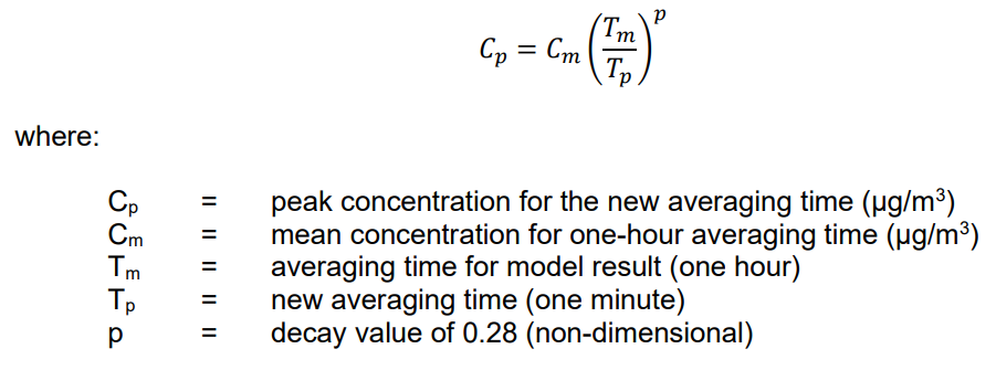
Sub-Hourly Objectives and Odour: Hourly model results are often converted to shorter averaging periods using scaling factors.

For example, 30-minute concentration ≈ hourly concentration × 1.21.

More generally, the scaling factor for air quality modelling can be approximated as follows (Ontario 2016):

Odour assessments may use a less stringent 99.5% tolerance, allowing rare events to be excluded. For 8,760 hourly observations per year, this typically removes the top 43 values at each receptor.

Sulphur and TRS Modelling: For odour and sulphur assessments, compounds such as:

• H₂S
• CS₂
• COS

may be modelled collectively as Total Reduced Sulphur (TRS) by summing the mass of each sulphur species before modelling.

The Bottom Line: A successful air quality assessment is not simply a model output. It demonstrates that the emissions assumptions, modelling approach, and predicted concentrations answer the regulatory question being asked and provide a defensible basis for regulatory decisions.

Air Quality Assessment Reports - Quick highlight from British Columbia

Emission rates can vary significantly over time, so matching the emission rate to the averaging period is critical for demonstrating compliance with air quality objectives.

• 1-hour concentrations: use the maximum emission rate observed during the entire modelling period.
• 8-hour, 24-hour, and annual concentrations: use the maximum emission rate for the corresponding averaging period (for example, the annual average emission rate for annual predictions).

In short, short-term assessments focus on worst-case emissions, while long-term assessments use period-specific average emission rates to reflect realistic operating conditions.

Compliance with air quality dispersion modeling in Saskatchewan

Air quality assessments show how a facility may affect the environment and provide the evidence regulators use to make decisions. This province is quite similar to Alberta.

The maximum pollutant concentrations

To support review and approval, reports should clearly present maximum predicted concentrations, distance from emission sources, tables and concentration map along with modelling assumptions and methodology

The goal is simple: make it easy for the reviewer to understand how the results were generated and whether air quality objectives are met.

For key modelling requirements maps and visualizations comparing results to air quality standards, consider this list of needs in the Saskatchewan guideline. 

• Use five consecutive years of hourly meteorological data.
• Record the maximum concentration at each receptor.
• Report results using tables and maps.
• Exclude hourly values above the 99.9th percentile where permitted.
• Run the model for each year and plot the highest annual average concentration at every receptor.

Maps should include:

• Concentration isopleths (lines of equal concentration)
• Areas where standards may be exceeded
• Topography
• Sensitive receptors
• At least 90% of the modelling domain

Models such as AERSCREEN predict hourly concentrations, while standards may apply to averaging periods ranging from minutes to years.

To compare results properly:

• Convert hourly predictions to shorter averaging periods using approved scaling factors.
• Convert units where necessary.

Refined dispersion models such as AERMOD predict hourly concentrations, but some air quality standards are based on shorter averaging periods, such as 30-minute or 10-minute values.

To compare model results with these standards, regulators recommend applying a time-scaling factor using a more general power-law equation. This converts a predicted 1-hour concentration into an equivalent shorter-term concentration, helping assess whether brief pollutant spikes could exceed air quality objectives.

The difficult assessments aren't necessarily the largest ones. They are often the ones where the operating scenario is uncertain, emissions vary substantially, several averaging periods apply, or the modelling produces exceedances that require interpretation.

Examples include:

• flare modelling
• odour
• intermittent sources
• unusual release configurations
• building effects
• NO₂
• TRS
• multiple operating scenarios
• regulatory uncertainty

That's where we come in...

At Calvin Consulting Group Ltd.,

A credible air quality assessment report must allow the reviewer to understand what was modelled, why it was modelled that way, and how the conclusions were reached.

Calvin Consulting Group Ltd. works on the difficult part of these assessments:

• determining what should be modelled,
• establishing defensible emission scenarios,
• selecting appropriate meteorology and modelling methods, and
• presenting the results in a form that regulators can review. 

We're here to solve your problems with air quality. Make compliance easy for your company. Barry at Calvin Consulting...

...can help. Let us handle this so you can focus on what you do best. 

In reviewing an assessment, I will often find that the most important question isn't whether AERMOD was run correctly. It's whether the scenario being modelled actually represents the facility.

A flare may operate for 15 minutes rather than an hour. A proposed stack may have changed height. A fuel-gas ratio may still be uncertain. A previous modelling case may no longer represent the current facility configuration. Those details can change the result more than another decimal place in the model output.

​Clean air is our Passion...Regulatory Compliance is our Business.

What the report doesn't tell you at first glance A model can be technically correct and still answer the wrong question.

Reading an air-quality assessment isn't about understanding every line of AERMOD output. It's about understanding the chain of assumptions that connects a facility's emissions to a regulatory conclusion.

Do you have concerns about air pollution in your area??

Perhaps modelling air pollution will provide the answers to your question.

That is what I do on a full-time basis.  Find out if it is necessary for your project.

Have your Say...

on the StuffintheAir         facebook page

Other topics listed in these guides:

The Stuff-in-the-Air Site Map

And, 

See the newsletter chronicle. 

Thank you to my research and writing assistants, and the author remains responsible for the content.

Before accepting the conclusions, I would check:

☐ Emission sources identified
☐ Emission rates documented
☐ Operating scenarios explained
☐ Meteorological dataset appropriate
☐ Terrain considered
☐ Model selection justified
☐ Receptors appropriate
☐ Averaging periods correct
☐ Concentration targets correctly identified
☐ Background concentrations addressed
☐ Maximum results clearly reported
☐ Exceedances explained
☐ Assumptions documented
☐ Conclusions supported by results

If you can't answer these questions from the report, the assessment may deserve a closer technical review.