- Air Homepage
- Air Quality Modelling Service
- Air Quality Dispersion Modelling
- Method of Variation of Parameters
Method of Variation of Parameters: How to Model Changing Emissions
How emission rates, stack conditions and operating conditions affect air quality dispersion modelling...where the Method of Variation of Parameters becomes important.
What happens when a facility does not operate the same way every hour?
A stack might operate at full production during one period and 50% during another. A flare might operate for only part of an hour. A blowdown can begin with a very high flow rate and then rapidly decline. Exhaust temperature and velocity can change with production. A storage pile may emit more particulate matter on a windy day than on a calm one.
Even the physical configuration of a release can matter. A raincap, horizontal exit, unusual release direction or nearby building can change how an emission enters the atmosphere. This is where the Method of Variation of Parameters becomes important.
In dispersion modelling, the objective is not simply to find an emission rate and put that number into AERMOD or CALPUFF. The model needs to represent a realistic operating condition, including the source parameters that influence how the emissions disperse.
And there is an important catch: The operating condition with the highest emission rate is not necessarily the condition that produces the highest ground-level concentration. That is one of the most important ideas to understand when developing model inputs.
What is the Method of Variation of Parameters?
The Method of Variation of Parameters allows source conditions to change rather than assuming that every hour of the model represents exactly the same operation.
Depending on the facility and the model, the parameters that vary can include:
- emission rate;
- emission factor;
- stack exit velocity;
- exhaust temperature;
- flow rate;
- production rate;
- source dimensions;
- operating hours; and
- other source-specific characteristics.
For a simple example, imagine a source with a maximum emission rate of 100 g/s. It might operate at:
- 100 g/s → 100% operation
- 75 g/s → 75% operation
- 50 g/s → 50% operation
- 0 g/s → shutdown
That seems straightforward. But suppose the exhaust velocity and temperature also decline as production falls.
The result is no longer simply a scaled version of the maximum case.
Lower exhaust velocity or temperature can reduce plume rise. In some situations, that can bring more of the plume down toward ground level and produce a higher predicted concentration even though the source is emitting less pollutant.
This is why good dispersion modelling is about much more than multiplying one number by a production factor.
Why the source parameters matter
Parameter
Why it matters
Emission rate
Determines how much pollutant enters the atmosphere
Stack height
Influences the distance available for dispersion before the plume reaches the ground
Exit velocity
Affects plume rise and the initial momentum of the release
Exit temperature
Affects buoyancy and plume rise
Stack diameter
Influences the release characteristics and relationship between flow and velocity
Release location
Determines where the plume begins relative to terrain and receptors
Operating hours
Determines when emissions occur
Hourly variation
This method of variation of parameters allows changing source conditions to be represented
Source geometry/orientation
Can matter for unusual releases such as horizontal or angled exits
The parameters also interact.
For example, emission rate, stack diameter and exit velocity should describe a physically consistent source condition. Increasing one value while leaving the others unchanged may produce a source that does not represent anything that could actually happen at the facility.
That is one of the first checks an experienced modeller makes.
Maximum emissions do not always mean maximum concentrations
This is where the subject becomes particularly interesting. Imagine a combustion source operating at 100% design load. It has:
- high emissions;
- high exhaust temperature;
- high exhaust flow; and
- high exit velocity.
Now imagine the same source operating at 50% load. The emission rate may be substantially lower, but so may the temperature and velocity.
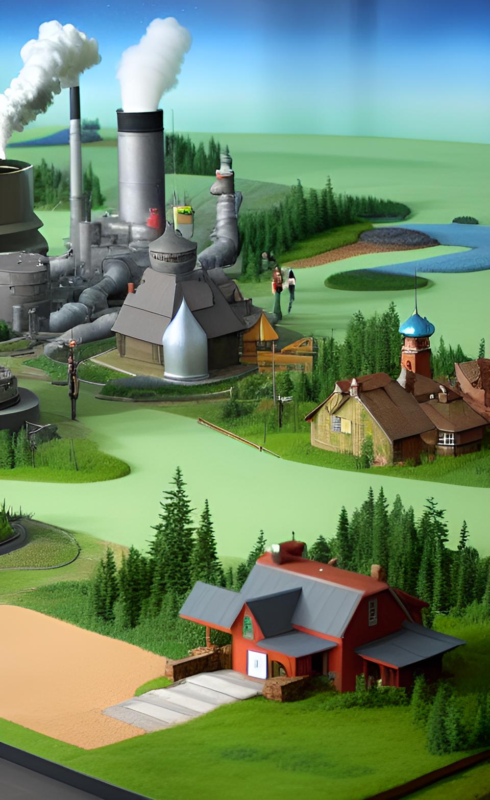 Modelling in prairie terrain
The first case has more pollutant while the second case may have less plume rise. And depending on the source and surrounding terrain, the second operating condition could therefore produce a higher concentration at ground level.
This is why regulatory modelling guidance in Western Canada recognizes the importance of considering different operating conditions rather than assuming that one maximum-emission scenario will always represent the worst case.
The practical question is: Which realistic operating condition produces the highest relevant concentration? That is the condition the modeller needs to find.
Where do the emission rates come from? The quality of the model can never be better than the information used to characterize the source.
Emission rates may come from several sources, depending on the facility:
- approved emission limits;
- continuous emission monitoring systems (CEMS);
- stack testing;
- manufacturer specifications;
- published emission factors;
- engineering calculations;
- emission-estimation tools;
- information from similar facilities; and
- process-specific calculations.
The best choice depends on the source and the purpose of the assessment.
Approved emission limits - An approved limit can provide an important regulatory basis for the model.
But a regulatory limit is not necessarily the same thing as the facility's normal operating emission rate. Before using it, the modeller should understand:
- what the limit represents;
- its averaging period;
- its units;
- whether it applies continuously or under specific conditions; and
- whether the value remains representative of the current facility.
A number copied directly from an approval is not necessarily a good model input.
CEMS: when the facility tells you what actually happened
Continuous emission monitoring can provide much more information than a single emission factor or stack test. Hourly CEMS data can reveal:
- when a source was operating;
- how emission rates changed;
- production patterns;
- periods of unusually high or low emissions; and
- relationships between emissions and operating conditions.
At Calvin, we have also worked with raw CEMS data, rather than simply taking a summary number from a report. That can be important when the modelling question depends on identifying representative operating conditions.
For example, an apparently simple question such as: What emission rate should represent normal operation? may require looking at the actual hourly record to determine how often the source operated, what range of emissions occurred and which periods are representative.
The answer can be quite different from simply selecting the largest number in the dataset.
Stack testing: useful, but remember what it represents
Stack testing provides site-specific information and can be extremely valuable. But a stack test is generally a measurement of what happened during the test.
The modeller still needs to consider whether those conditions represent:
- typical operation;
- maximum operation;
- a particular production level;
- a particular fuel;
- a particular control-equipment condition; or
- some other specific operating state.
A good stack test can be excellent model input. A good stack test interpreted in the wrong context can still produce a poor model.
Manufacturer data and emission factors
For new facilities, manufacturer specifications may be the best information available. Published emission factors can also be useful where site-specific information does not exist.
 Modeling and measuring emissions
The key question is always: How closely does this information represent the facility we are actually modelling?
Equipment may operate differently from the conditions under which a manufacturer specification or emission factor was developed.
That is where professional judgment becomes important.
A modeller should be able to explain not only where the number came from, but why it is appropriate for this facility and operating condition.
Don't vary the emission rate and ignore everything else
Perhaps the most common mistaken method of variation of parameters is treating production rate and emission rate as though they were the only things that change.
They may not be. A change in production can also affect:
- exhaust temperature;
- exhaust velocity;
- flow rate;
- fuel use;
- pollution-control performance;
- source configuration; and
- operating hours.
The model should therefore represent a coherent operating condition, rather than a collection of independently scaled numbers. For example:
50% emission rate + 100% exhaust velocity + 100% exhaust temperature
...may or may not describe a real operating condition. The modeller needs to find out.
Unusual releases: when standard stack assumptions aren't enough
Some sources don't behave like ordinary vertical stacks. Examples include:
- raincapped stacks;
- horizontal exits;
- angled or directional releases;
- high-velocity vents;
- pressure-relief devices;
- blowdown releases;
- flares; and
- releases influenced strongly by nearby structures.
These cases can require additional thought because the way the material initially enters the atmosphere can affect the predicted concentrations.
 Ground-level concentrations in the city
Raincaps and horizontal exits - A source that is not exhausting vertically into the atmosphere cannot automatically be treated as an ordinary vertical stack.
The direction of the release, the momentum of the discharge and the surrounding physical environment may all affect the initial plume behaviour. The correct modelling treatment depends on the release and the capabilities of the selected dispersion model.
Buildings are a related but slightly different issue - Buildings do not technically represent a method of variation of parameters in the same way that emission rate or temperature does.
However, they can dramatically affect what happens after the release leaves the source. Building wake and downwash can bring an elevated plume toward ground level much sooner than it would otherwise reach it.
For unusual high-velocity or directional releases, the modeller therefore needs to think about both:
- How does the material leave the source? and
- What happens when it encounters the surrounding structures?
Those questions can matter more than simply adjusting the emission rate.
Blowdowns and flaring: when the parameters change rapidly
Blowdown events are a particularly good example of why the Method of Variation of Parameters matters.
A blowdown does not necessarily emit at one constant rate for its entire duration. The flow can begin very high and then decline rapidly.
For flare and blowdown assessments, Calvin has experience using AERflare to calculate appropriate parameters for representative flow conditions and then incorporating those conditions into dispersion modelling. A simplified way of thinking about the process is:
Blowdown event
↓
Flow changes with time
↓
Source parameters change
↓
Representative modelling conditions are developed
↓
↓
Results are evaluated using the relevant event duration and regulatory averaging period
For some blowdown assessments, Calvin represents the changing event using three representative flow rates (i.e., a high, middle and lower flow condition) and then evaluates which produces the controlling result when the duration and applicable averaging period are considered.
This is a good example of why simply modelling the highest instantaneous flow for the entire event may not provide the most meaningful answer.
The question is not merely: What was the highest flow? It is: What combination of flow, source parameters and event duration produces the relevant worst-case concentration?
Flare logs can be more useful than a single design number. Actual flare operation can also vary considerably.
Flare logs can provide information about:
- how often flaring occurred;
- how long it lasted;
- operating conditions;
- flow characteristics; and
- recurring events or schedules.
Where appropriate, Calvin has reviewed flare logs to help establish representative operating conditions. That can be especially useful when the goal is to model something that actually happens at the facility rather than a theoretical maximum that may almost never occur.
The same principle applies to CEMS data: Real operating data can reveal patterns that are invisible in a single maximum value.
Storage tanks are another special case
Tank emissions are not always measured directly. Calvin calculates tank emissions using established algorithms based on EPA methods, including approaches historically associated with the TANKS software.
The important point is that tank emissions can depend on more than the amount of material stored. Factors can include:
- tank design (including colour);
- liquid characteristics;
- temperature;
- throughput;
- fill level;
- breathing losses;
- working losses; and
- other operating conditions.
The modeller therefore needs to identify the appropriate calculation method and make sure the resulting emissions are consistent with the actual facility.
Tank modelling is a good example of the broader principle: The source representation comes first. The dispersion model comes second.
Comparing today's facility with yesterday's data
Existing facilities can provide another valuable source of information. Before accepting a new set of source parameters, Calvin may compare recent and historical:
- AEIR submissions;
- NPRI submissions;
- AER licence information;
- approval information; and
- other available operating data.
This can reveal changes that are easy to miss when looking at one document in isolation.
For example:
- Has the stack height changed?
- Has the equipment been replaced?
- Has the permitted emission rate changed?
- Has production increased?
- Has the source disappeared from one inventory but remained in another?
- Do the reported values remain consistent from one year to the next?
These comparisons are not merely administrative housekeeping. They can help determine whether the model is describing the facility that exists today.
Choosing representative operating conditions
A good assessment does not necessarily model every possible combination of parameters; that would be an excessive method of variation of parameters. That could result in an enormous number of scenarios without improving the answer.
Instead, the modeller should identify the operating conditions that are both realistic and potentially important to the modelling result. For example:
Operating condition
Why it may matter
100% design load
May produce the highest emission rate
Reduced load
May reduce plume rise and increase ground-level concentrations
Typical operation
May better represent routine exposure or annual conditions
High production with unusual stack conditions
Could produce an unexpected maximum
Intermittent operation
May affect short-term averages
Blowdown/flaring event
May involve rapidly changing source parameters
Shutdown/startup
May have unusual emissions or source conditions
The model should be designed around the regulatory question, not simply around the desire to model more cases.
Four ways to represent changing emissions
There is no single method that is best for every source.
Constant maximum rate - The source is represented at a conservative maximum relevant rate.
 Environmental modelling in Alberta
This can be appropriate for some regulatory assessments where a maximum credible continuous operating condition is the question.
Representative operating scenarios - Several discrete conditions are modelled separately. This is useful when a facility has clearly defined operating states.
Hourly variation - Emission rates and, where appropriate, other source parameters are allowed to change hour by hour. This can be particularly useful where CEMS or reliable operating data are available.
Event-based modelling - A short-duration or transient event is represented using source conditions appropriate to the event. Blowdowns and some flaring situations are examples.
The most appropriate approach depends on the source, available information, modelling system and regulatory objective.
What the Western Canadian guidelines have in common
BC, Alberta, Saskatchewan and Manitoba each provide guidance for developing emissions information and dispersion model inputs.
The details differ, but the underlying principle is similar: The model should be based on representative, defensible source information and appropriate operating conditions.
 Use realistic data to keep BC beautiful
This is why it is useful to understand the guidance in each province rather than simply copying an input approach from another project.
British Columbia - BC provides detailed guidance on emission rates, operating conditions, variability, source parameters and the use of available site-specific information.
Alberta - Alberta projects commonly require detailed source information, emission rates, operating conditions and the method used to quantify those values. The assessment needs to represent the facility and scenarios relevant to the regulatory question.
Saskatchewan - Saskatchewan guidance addresses changing emission rates and source parameters and recognizes that hourly variation can be used as a method of variation of parameters.
Manitoba - Manitoba modelling guidance likewise emphasizes understanding the facility, identifying its sources and developing representative emission rates and source parameters.
The provincial guidance provides the framework. The modeller still has to determine how that framework applies to the particular facility.
The main lesson
The Method of Variation of Parameters is not simply a way to tell AERMOD or CALPUFF that a source emits 50% instead of 100%. It is a way of asking a more important question: What is the source actually doing when the atmosphere is being exposed to it?
A good dispersion model represents that physical reality as closely as the available information allows.
Sometimes the answer comes from an approval, it comes from a stack test, it comes from CEMS data, flare logs or operating schedules. Or sometimes it requires comparing several years of AEIR and NPRI information.
For tanks, it may require emissions calculations. For blowdowns, it may require AERflare and several representative flow conditions.
And for unusual releases, the modeller may need to examine the physical release configuration itself (including exit direction, raincaps, high-velocity discharge and nearby buildings.)
The best model input is often more than just the biggest number. It is the parameter set that best represents the physical operating condition that matters to the modelling question.
Need help deciding what belongs in the model?
The difficult part of dispersion modelling is often not running the model. Usually it's deciding what the model should represent.
Calvin Consulting Group has more than 30 years of experience developing and reviewing air-quality dispersion models for industrial facilities across Western Canada.
We work with:
- regulatory approvals,
- emissions inventories,
- CEMS data,
- flare records,
- operating information,
- emission calculations and
- unusual source configurations
...to develop model inputs that are technically defensible and appropriate for the question being asked.
That can mean identifying a representative operating condition, reconciling conflicting historical data, determining whether hourly variation is warranted, or deciding that an apparently complicated modelling problem does not actually require a more complicated model.
Before asking the model for an answer, make sure you have given it the right question—and the right source parameters.
Contact Barry at Calvin Consulting Group to discuss an air quality modelling assessment or a source-parameter problem you need to resolve.

Let's talk about your air quality goals and how dispersion modeling can help. Let's make the world a cleaner, healthier place together.
Clean air is our Passion...Regulatory Compliance is our Business.
A practical checklist for source parameters
Before finalizing the model inputs, ask:
Emissions
- Where did each emission rate come from?
- Is the information current?
- What averaging period does it represent?
- Is it a limit, measured value, estimate or engineering calculation?
Operating conditions
- What does the source actually do at 100%, 75%, 50% and other relevant loads?
- Do emission rates change with production?
- Do temperature, velocity or flow also change?
Source geometry
- Is the release vertical?
- Is there a raincap?
- Is it horizontal or angled?
- Is it a flare, relief valve, blowdown or other unusual release?
Data validation
- Do recent AEIR and NPRI values make sense compared with historical submissions?
- Do licence and approval values agree with the model inputs?
- Are CEMS or operating logs available?
Time variation
- Is the source continuous or intermittent?
- Would hourly variation provide a better representation?
- Does the event duration matter to the applicable averaging period?
Physical plausibility
- Do the emission rate, diameter, flow and velocity form a physically consistent source?
- Do the selected parameters describe a condition that could actually occur?
Modelling judgment
- Which condition is expected to produce the highest relevant concentration?
- Have unusual but credible conditions been considered?
- Is additional modelling likely to change the decision?
Related air-quality modelling resources
Understanding variable parameters is closely connected to several other parts of an air-quality assessment:
Air Quality Modelling QA/QC: A practical checklist for checking emissions, stack parameters, buildings, meteorology, terrain, receptors and model configuration.
Different Operating Conditions (see above): How normal, maximum, reduced-load and unusual operating conditions are selected for modelling.
AERflare and Flare Modelling: How flare emissions and changing flare conditions can be represented in dispersion modelling.
Building Downwash: How buildings can alter the dispersion of elevated releases.
Air Quality Assessment Reports: How source inputs ultimately become predicted concentrations and regulatory conclusions.
AERMOD vs. CALPUFF: How the choice of dispersion model affects the way source and meteorological information are represented.
Land Use and Land Cover: How the surrounding landscape affects dispersion modelling.
Long-Range Transport and Modelling Domains: How far the assessment needs to extend beyond the facility.
Recent Articles


-
Natural Gas Leak Detection: Does YOUR Facility Need it?
Sep 28, 26 08:40 AM
 It's important for industries, especially in the energy sector, to have a natural gas leak detection program. It's often required by law.
 -
Computers in Meteorology | How Would they Help You?
Sep 26, 26 09:40 PM
 Computers in meteorology help us keep track of atmospheric data and make predictions.
 -
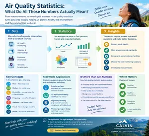
Air Quality Statistics: What Do All Those Numbers Actually Mean?
Sep 21, 26 12:00 AM
 How are air quality statistics used to understand pollution, design monitoring programs, estimate emissions and make environmental decisions?
What an experienced modeller looks for
When reviewing a set of source inputs, I don't start by asking whether every cell in the model input file has been filled in.
I start by asking whether the source makes physical sense.
Do the parameters belong together? - Does the emission rate correspond to the stated operating condition? Does the flow make sense with the stack diameter and exit velocity? Does the temperature correspond to the selected load?
Is the source information current? - Does it agree with the most recent AEIR, NPRI and approval information? If the information differs from historical data, is there a reason?
Is the condition actually realistic? - A theoretical maximum can be useful, but it should not automatically be assumed to represent normal operation.
Could a lower emission rate create a higher concentration? - This is particularly important where stack conditions change with load or where terrain or building effects are significant.
Does the release geometry make sense?
- Is the source truly vertical?
- Is there a raincap?
- Is the release horizontal or angled?
- Is it a high-velocity vent?
- Does the surrounding building environment need particular attention?
Is the source intermittent? - If so, should the model represent the source as continuously operating, through hourly variation, or as a discrete event?
What is the regulatory question? - A source representation that is appropriate for one averaging period may not be the right representation for another. The modelling approach should follow the question.
Do you have concerns about air pollution in your area??
Perhaps modelling air pollution will provide the answers to your question.
That is what I do on a full-time basis. Find out if it is necessary for your project.
Have your Say...
on the StuffintheAir facebook page
Other topics listed in these guides:
The Stuff-in-the-Air Site Map
And,
Thank you to my research and writing assistants, and the author remains responsible for the content.
Common mistakes in variation of parameters
Using the maximum emission rate for everything - This may be conservative, but it can produce an unrealistic representation of some operating conditions and does not necessarily identify the highest concentration.
Changing the emission rate but not the stack parameters - Production changes can affect temperature, velocity and flow.
Treating a permit limit as though it were a measured operating rate - The two may be very different.
Choosing the largest value in a CEMS dataset without understanding the data - A maximum hourly value may represent an unusual event rather than a representative operating condition.
Ignoring operating schedules - An intermittent source cannot always be treated as though it operates continuously.
Treating unusual releases like ordinary stacks - Raincaps, horizontal exits, directional vents, relief devices and blowdowns may require specialized treatment.
Ignoring historical discrepancies - Changes between AEIR, NPRI, licence and other records can reveal changes in the facility or problems with the underlying data.
Modelling every imaginable scenario - More scenarios do not automatically mean a better assessment.
The goal is to identify the scenarios that can actually affect the decision.
Most Popular Pages on this Website:
Pictures of Global Warming
- See photos, cartoons, charts, graphs and a few surprises.
Clouds
- Don't know a cumulus from a stratus? Check here.
Causes of Global Warming
- It's not always obvious.
Calgary Alberta Weather
- Example of Canadian Goodness.
Thermometers
- Our favourite weather instrument.
- Home
- Contact Us
- Free E-zine Back Issues
- Privacy Policy
- Site Map - I'll help find something good.

By Barry Lough, P.Met., EP (Environmental Professional)
Text copyright © 2003-2026 Stuff in the Air.com
BACK TO TOP - Hit your 'Home' Key