How Secondary Pollutants of Air Pollution Are Modelled

What happens when the pollutant you care about isn't the pollutant that came out of the stack?

A dispersion model is easiest to understand when the pollutant comes directly from a source. 

A stack emits SO₂. The model transports it through the atmosphere. A receptor receives a predicted concentration.

Predicting secondary pollutants

But what happens when the pollutant you are trying to predict forms after the emission has left the stack? Now the problem gets considerably more interesting.

Some of the particulate matter in the atmosphere is emitted directly. Other particulate matter forms later through chemical reactions involving gases released by industrial facilities, transportation, agriculture and other sources.

Ozone is another familiar example. A facility does not simply emit 'ozone' from a stack and watch it drift downwind. Ozone can form, react, increase or decrease as precursor pollutants interact with the atmosphere.

This is the world of secondary Pollutants of Air Pollution.

And it raises a deceptively simple question: How do you model something that doesn't exist yet when the emissions leave the source?

Primary versus secondary pollutants

The distinction is fundamental.

Primary pollutants - These are emitted directly by a source. Examples include:

• SO₂;
• NO;
• NO₂;
• directly emitted particulate matter; and
• many individual gases and vapours.

Secondary pollutants - These form after emissions enter the atmosphere. Examples include:

• secondary sulphate particulate matter;
• secondary nitrate particulate matter;
• ozone; and
• some forms of secondary organic aerosol.

The difference can be summarized like this:

Primary pollutant:

Source → atmosphere → receptor

Secondary pollutant:

Source → atmosphere → chemical reactions → new pollutant → receptor

That's why secondary Pollutants of Air Pollution can require a very different modelling approach from a conventional stack assessment.

Follow the pollutant, not just the plume

Imagine releasing sulphur dioxide into the atmosphere. At the stack, the emission is SO₂. A few kilometres downwind, some of that material may have reacted.

Farther away, the mixture may contain other sulphur species. Eventually, some of that material can be deposited onto the ground or incorporated into particles.

The pollutant has effectively changed identity while travelling. The same general idea applies to nitrogen chemistry.

NO and NO₂

↓

atmospheric reactions

↓

oxidized nitrogen species

↓

secondary particulate matter and/or deposition

The actual chemistry is considerably more complicated than these sketches, but this is the reason secondary pollutants of air pollution cannot always be treated as passive pollutants simply carried from a stack to a receptor.

Why secondary PM₂.₅ is particularly difficult

Secondary particulate matter is really the core of this subject. PM₂.₅ is not a single chemical substance. It can contain many different components.

Some PM₂.₅ is emitted directly from sources. Some forms from precursor gases after they have entered the atmosphere. 

Important secondary components can include sulphate, nitrate and ammonium, as well as secondary organic material under appropriate atmospheric conditions. That creates several questions for the modeller:

• How much precursor was emitted?
• Where did it travel?
• What did it react with?
• How quickly did it react?
• What other emissions were present?
• What were the atmospheric conditions?
• How much of the resulting material remained airborne?
• How much was removed by deposition?

That is a much bigger problem than simply entering a PM₂.₅ emission rate into a dispersion model.

Can AERMOD model secondary pollutants of air pollution?

This is an excellent question, and the answer is more nuanced than a simple yes or no.

AERMOD is extremely useful for modelling the primary component of particulate matter and other pollutants emitted directly from sources. It can also handle certain atmospheric transformation and deposition processes.

Air quality assessments

But AERMOD should not be treated as a complete regional photochemical model for secondary PM₂.₅ or ozone formation. That distinction matters.

For secondary pollutants of air pollution, the modeller may need to account for chemical reactions involving emissions from many sources and the background atmosphere.

Modern U.S. EPA guidance recognizes that evaluating secondary ozone and PM₂.₅ may require chemical transport models that simulate how pollutants form, break down and move through the atmosphere. For single-source secondary PM₂.₅, a tiered approach is used, ranging from established screening relationships to detailed, case-specific chemical transport modelling.

So AERMOD can be an important part of the overall assessment. It is not automatically the entire answer.

Why a conventional dispersion model can run into trouble

Suppose an industrial facility emits a precursor gas that contributes to secondary PM₂.₅. Immediately after release, the plume may be relatively narrow.

As it travels, it spreads. At the same time, chemical reactions begin.

Now imagine trying to represent that process with a large regional grid. The individual plume may be much narrower than the grid cell.

If the model simply spreads the emissions uniformly across that cell, important near-source information can be lost. This is one reason advanced regional modelling can require specialized techniques.

The plume-in-grid problem

A regional chemical-transport model typically divides the atmosphere into three-dimensional grid cells. That's powerful because it allows chemistry and transport to be represented across a large region.

But there is a catch: A grid cell can be much larger than an individual industrial plume.

Imagine a large square representing one regional grid cell. Inside it is a much narrower plume from a stack.

If the model immediately distributes the source emissions across the entire square, the initial plume structure disappears.

A plume-in-grid (PIG) approach can preserve a more detailed representation of the individual plume within the regional grid while it is still too narrow to be represented realistically by the grid alone.

That can be important when modelling secondary pollutants of air pollution because chemical reactions can begin while the plume is still relatively concentrated.

British Columbia has specifically addressed plume-in-grid methods for secondary pollutant modelling and recognizes the difficulty of resolving individual source plumes within regional grid models.

Why chemistry matters

Secondary formation depends on what the pollutant encounters after release. The atmosphere is not an empty container. It contains:

• oxygen;
• ozone;
• water vapour;
• ammonia;
• oxidants;
• other pollutants;
• particles; and
• emissions from other sources.

Meteorology matters too. Temperature, sunlight, cloud water, wind and atmospheric stability can all influence chemical transformation and transport. This means an evaluation of secondary pollutants of air pollution can require considerably more information than a conventional AERMOD assessment.

The problem is no longer simply: How far did the plume travel? It becomes: What happened to the plume while it travelled?

Ozone is a particularly good example - Ground-level ozone is a secondary pollutant.

Its chemistry depends on precursor emissions, particularly nitrogen oxides and volatile organic compounds, together with atmospheric conditions. That means a facility can contribute to an ozone problem without directly emitting ozone.

The same basic principle applies to secondary PM₂.₅. The facility may emit precursors. The atmosphere does the chemistry. The eventual pollutant can appear somewhere downwind. This is why secondary pollutants of air pollution can become a regional rather than purely local modelling problem.

Where CALPUFF fits

CALPUFF occupies an interesting position between conventional Gaussian plume modelling and full regional photochemical grid modelling. It can represent:

• non-steady-state transport;
• time- and space-varying meteorology;
• changing plume trajectories;
• chemical transformation;
• deposition; and
• transport over larger distances.

For some applications, that makes CALPUFF useful for investigating secondary particulate formation and related regional processes.

But CALPUFF should not be presented as a universal answer either. The suitability of the chemistry, meteorology and model configuration depends on the assessment. 

In other words: CALPUFF's ability to represent chemistry does not automatically make every CALPUFF secondary-pollutant assessment defensible. The quality of the inputs and the appropriateness of the chemical mechanism still matter.

CALPUFF versus a photochemical grid model - There is a useful difference between the approaches.

CALPUFF Follows puffs emitted from identified sources through changing meteorological conditions. And this can be useful when individual source plumes and their transport are important.

Photochemical grid models such as CMAQ and CAMx divide the atmosphere into a three-dimensional grid and simulate the chemical and physical processes occurring within it. They are particularly useful when:

• many sources interact;
• secondary formation is important;
• regional transport matters; or
• ozone and secondary PM₂.₅ need to be assessed over a broad area.

For complex secondary ozone and PM2.5 assessments, the EPA recommends photochemical grid models because they can represent a dynamically changing chemical and physical atmosphere. Lagrangian approaches can also be appropriate in some cases.

So the question is not: 'Which model is most advanced?', it is: Which model can represent the processes that matter to this assessment?

What data does secondary-pollutant modelling need?

This is where the problem can become much larger than expected. Depending on the assessment, the modeller may need:

Emissions - Detailed precursor emissions from the project and potentially other important sources.

Chemical speciation - Knowing the total mass may not be enough. The model may need to know the chemical form of the emissions.

Meteorology - Wind, temperature, stability, cloud and other variables needed to represent transport and atmospheric chemistry.

Background chemistry - Secondary formation depends partly on what is already present in the atmosphere.

Terrain and land use - These can affect meteorology and therefore transport.

Boundary conditions - Regional chemical-transport models may require information entering the modelling domain from outside it.

Monitoring data - Observations can be important for evaluating whether the model is adequately representing actual atmospheric conditions.

This is one reason that an apparently simple request to model secondary PM₂.₅ can become a major technical exercise.

Modelling secondary PM₂.₅ is not the same as modelling primary PM₂.₅

This distinction is worth remembering.

Primary PM₂.₅ - The particles already exist when they leave the source. The modeller needs to know their emission rate and physical properties, including particle size distribution where deposition or aerodynamic behaviour makes that important.

Secondary PM₂.₅ - Some of the particles form later from gaseous precursors. The modeller needs to understand the chemical transformation as well as transport and removal.

A single assessment can contain both. A facility might directly emit particulate matter while also emitting SO₂, NOx, VOCs or other precursors that contribute to secondary PM₂.₅. The two contributions should not automatically be treated as though they were the same thing.

What about NO₂?

Nitrogen dioxide is an interesting borderline case because it can be formed rapidly in the atmosphere after emission of NO. For routine industrial assessments, AERMOD has established approaches for estimating NO₂ from NOx emissions, including methods such as PVMRM and OLM.

But NO₂ modelling should not be confused with full regional secondary-pollutant modelling. The chemistry and time scales are different. The fact that AERMOD can represent an important atmospheric transformation does not mean it is a general photochemical model.

That distinction is particularly important when discussing secondary Pollutants of Air Pollution.

Western Provinces

British Columbia: a particularly useful example - British Columbia has developed separate modelling guidance for photochemical assessments involving secondary pollutants.

In British Columbia, Alberta and Saskatchewan

The province's current modelling resources identify a Lower Fraser Valley Photochemical Modelling Guideline for estimating project impacts on secondary pollutants such as ground-level ozone and secondary particulate matter.

BC also maintains its general air-quality dispersion modelling guideline and a separate NO₂ modelling guide.

That structure is revealing. It reflects a basic modelling principle: Different atmospheric questions can require different modelling tools. A conventional dispersion assessment and a regional photochemical assessment should not automatically be treated as the same exercise.

Alberta: when does this become an issue? - Alberta has a history of regional air-quality and secondary PM₂.₅ modelling, including work in the Edmonton region and the oil sands region.

Photochemical modelling has been used to investigate regional PM₂.₅ formation, source contributions and atmospheric chemistry. 

For an individual industrial project, however, secondary-pollutant modelling is much less routine than ordinary refined dispersion modelling.

That distinction matters for anyone reading this page and wondering: Do I need CMAQ? Probably not—unless the project and applicable regulatory framework give you a reason.

A secondary-pollutant assessment can require substantial emissions inventories, chemical inputs, meteorology, background information and model evaluation. Before embarking on that exercise, it is worth determining exactly what question the assessment needs to answer.

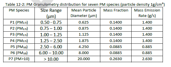
Saskatchewan: particulate matter and particle properties - Saskatchewan's modelling guidance also illustrates an important point about particulate matter.

Not all particles behave identically. Particle characteristics such as:

• diameter;
• density;
• mass fraction; and
• aerodynamic properties

...can affect dispersion and deposition.

These properties are particularly relevant when modelling primary particulate emissions and deposition. They should not be confused with the separate problem of determining how gaseous precursor emissions chemically form secondary PM₂.₅.

Keeping those two problems separate makes the modelling approach much easier to understand. You can use this table for CALPUFF deposition calculations:

What an experienced modeller asks before choosing a model

Secondary-pollutant modelling is specialized enough that the first question should not be: 'Which software package should we buy?'

At Calvin, we'd start with the assessment itself.

What is the pollutant of concern? Secondary PM₂.₅? Ozone? Nitrogen compounds? Acidifying deposition? Something else?

What is the scale? A few kilometres around one facility? A regional airshed? Multiple interacting facilities? 

What are the precursor emissions? Which sources matter? How large are their emissions? How are those emissions distributed?

What chemistry is important? What reactions have to be represented? What atmospheric constituents are needed?

What observations are available? Do we have enough meteorological and chemical data to support the model?

What does the regulator actually require? Is a full photochemical model required? Is an existing technical relationship sufficient? Would a screening analysis answer the question?

Does the additional complexity change the decision?

This is the most important question of all. A more sophisticated model is useful only when its additional capabilities answer a question that matters.

Is it necessary to model secondary pollutants?

Why this is not a good modelling problem to solve by trial and error

With conventional AERMOD modelling, it is tempting to think: 'I'll put together an input file, run it, look at the result and adjust it until it looks sensible.'

That approach becomes much more problematic when chemistry is involved. Now the modeller may be making decisions about:

• precursor speciation;
• chemical mechanisms;
• reaction rates;
• background concentrations;
• boundary conditions;
• meteorology;
• spatial resolution;
• plume treatment;
• deposition; and
• model performance.

A technically correct calculation can still represent the wrong physical system. That is one reason secondary-pollutant modelling is an area where specialist review is particularly valuable.

The Calvin perspective

This is a relatively esoteric area of air-quality modelling. Secondary PM₂.₅ formation is not a routine component of the industrial projects Calvin Consulting performs.

In fact, we have not yet taken on a project where modelling secondary particulate formation was required as the central assessment task.

That is worth saying plainly. It does not mean we cannot undertake one.

Our core expertise in industrial emissions, dispersion modelling, source characterization, AERMOD, CALPUFF, meteorology, terrain and regulatory assessment gives us the foundation to investigate a project requiring this type of work.

Where necessary, that would mean researching the applicable guidance and modelling methodology, determining what data are required, selecting an appropriate modelling system and working through the additional chemistry and validation requirements.

We would not pretend that a conventional AERMOD model can answer a question that requires a regional photochemical model. Nor would we assume that the existence of a sophisticated model means it has to be used.

The first job is to establish what the assessment needs to demonstrate. The second is to determine how to model it.

The main lesson

Secondary pollutants turn a familiar dispersion problem into something much more complicated.

The emissions leave the facility. The atmosphere transports them. Chemical reactions change them.

Good environmental science for the benefit of our children.

New pollutants form. Those pollutants continue to move and react. Some are deposited. Some remain airborne.

The final concentration or deposition is therefore the product of emissions, transport, chemistry and removal, not simply the emission rate at the stack. That is why secondary Pollutants of Air Pollution are among the more specialized problems in air-quality modelling.

And it explains why the first question should not be: 'Can AERMOD do this?' or even: 'Should we use CALPUFF?'

The better question is: What processes do we need to represent to answer the environmental and regulatory question? Once that is clear, the appropriate modelling approach becomes much easier to identify.

Need to investigate a secondary-pollutant issue?

A request to evaluate secondary PM₂.₅ or ozone can sound simple until the modeller starts listing the information required.

• What are the precursor emissions?
• What chemistry matters?
• What happens in the background atmosphere?
• How large does the modelling domain need to be?
• Is the individual plume important?
• Can existing modelling or published relationships answer the question?
• Or is a full chemical-transport model required?

These are not usually questions that can be answered confidently by picking a model from a software list.

Calvin Consulting's core business is industrial air-quality dispersion modelling and specialized secondary-pollutant assessments have been a relatively small part of our work to date. Where a project requires one, however, we have the technical background and capability to investigate the methodology, assemble the required information and undertake the assessment.

Sometimes the most useful modelling decision is knowing that a conventional model is enough. Sometimes it is knowing when it isn't.

Before investing in a complicated secondary-pollutant modelling exercise, contact Calvin Consulting Group to discuss what the project actually needs to demonstrate and what modelling approach can defensibly answer it.

And let Calvin Consulting take the complexity out of your air quality modelling needs.

​Clean air is our Passion...Regulatory Compliance is our Business.

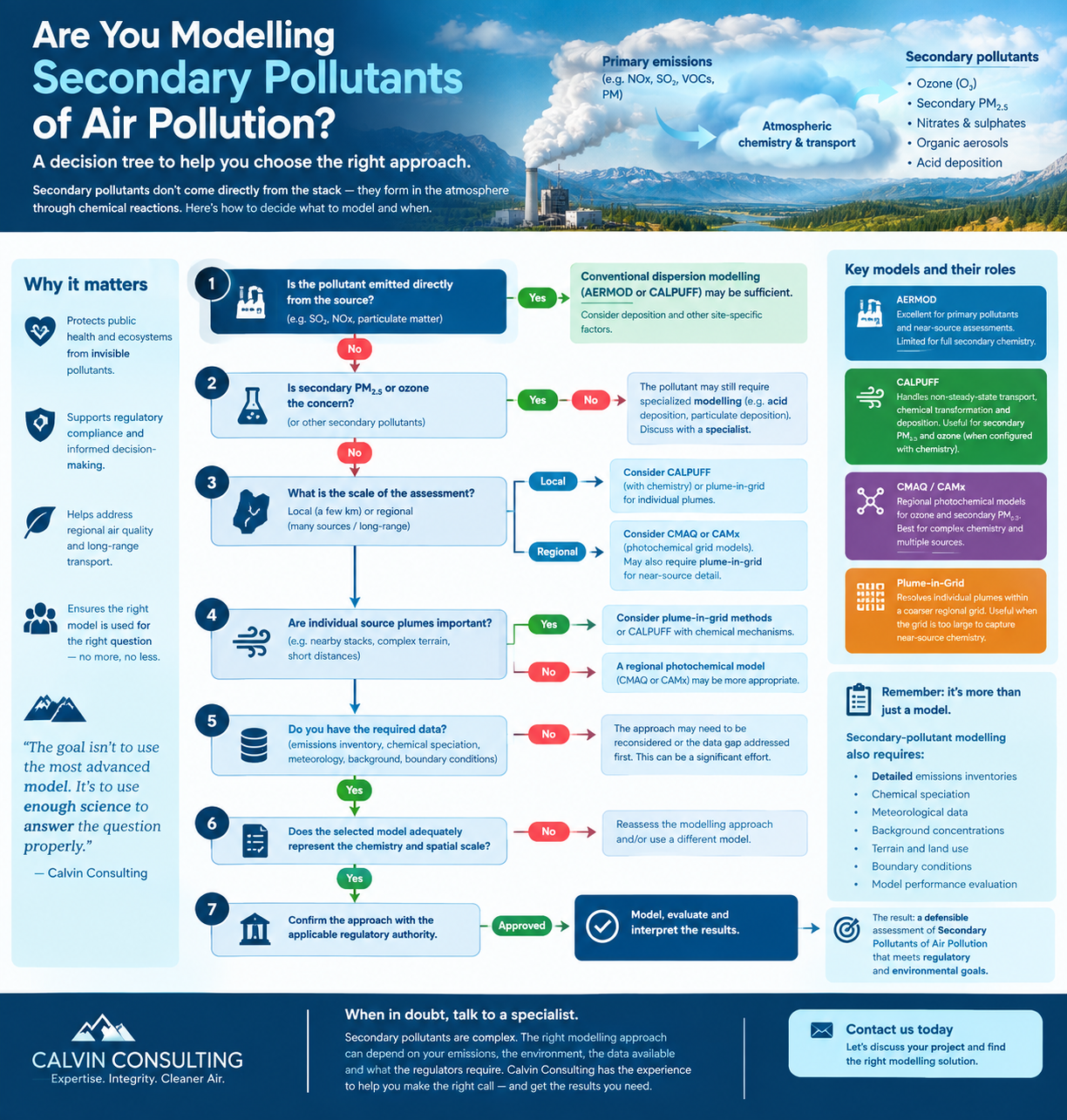
A practical secondary-pollutant decision path

1. Is the pollutant emitted directly?

Yes - Start with conventional dispersion modelling appropriate to the source and regulatory question.

No, or secondary formation is potentially important

↓

Is secondary PM₂.₅ or ozone the concern?

↓

Is the assessment local or regional?

↓

2. Are individual source plumes important?

Yes - Consider a Lagrangian or plume-in-grid approach where appropriate.

No / many sources interact - 

Consider a regional photochemical grid model.

↓

3. Are the required emissions, meteorology and chemical data available?

No - The modelling approach may need to be reconsidered or the data gap addressed first.

Yes - Does the selected model adequately represent the chemistry and spatial scale?

↓

Confirm the approach with the applicable regulatory authority

↓

Model, evaluate and interpret the results

-

This decision path is deliberately conservative.

The right answer may be that a highly sophisticated model is required.

It may also be that it isn't.

Do you have concerns about air pollution in your area??

Perhaps modelling air pollution will provide the answers to your question.

That is what I do on a full-time basis.  Find out if it is necessary for your project.

Have your Say...

on the StuffintheAir         facebook page

Other topics listed in these guides:

The Stuff-in-the-Air Site Map

And, 

See the newsletter chronicle. 

Thank you to my research and writing assistants, and the author remains responsible for the content.

Common mistakes with secondary pollutants

1. Treating secondary PM₂.₅ as though it were all directly emitted: PM₂.₅ can contain both primary and secondary components.
2. Assuming AERMOD solves every PM₂.₅ problem: It is extremely useful for primary dispersion, but full secondary formation can require chemical-transport modelling.
3. Assuming CALPUFF automatically solves secondary chemistry: Its chemical capabilities still depend on the selected mechanism, inputs and application.
4. Choosing a model because it sounds advanced - 'Advanced' is not a modelling objective.
5. Ignoring background chemistry - Secondary formation depends on what is already present in the atmosphere.
6. Underestimating the emissions inventory - A regional chemistry problem can require much more than the project's own stacks.
7. Using a regional grid that cannot resolve the plume - This is one reason plume-in-grid methods exist.
8. Treating primary and secondary PM₂.₅ as the same thing - They are related but physically different modelling problems.
9. Starting the chemistry before understanding the regulatory question - This is a particularly expensive mistake.